We can use the GNU Octave tool to acquire samples from the RedPitaya and then do basically whatever processing we want.

The function acquire shown below is a simple GNU Octave script that loads samples from the RedPitaya and returns the sample vectors as a two-column matrix. As input it needs the RedPitaya IP address, the number of samples to acquire (max. 16384), the optional decimation factor and averaging selection.

As I’m running Octave on windows the PuTTy tool must also be installed to be able to transfer data over an SSH connection.

%> @brief Acquire samples from Red Pitaya.
%>
%> Note: PuTTy must be installed and the path to the PuTTY
%> installation folder must be in included into the windows
%> search path.
%>
%> @param ipAddress Red Pitaya IP address (or hostname).
%> @param nSamples Number of samples to capture.
%> @param decimationFactor Decimation factor (1,8,64,1024,8192,65536).
%> @param averagingIsEnabled If true, enable averaging when decimating.
%> @retval data Acquired data (two columns, channels 1 and 2).
function data=acquire(ipAddress,nSamples,decimationFactor,averagingIsEnabled)

DATA_FILE = 'data.txt';

if puttyIsNotInstalled
   disp('plink.exe not found, please install PuTTy!');
   return
end

setAveragingRegister(ipAddress, averagingIsEnabled);
acquireDataIntoFile(ipAddress,DATA_FILE,nSamples,decimationFactor);
data = loadDataFromFile(DATA_FILE);
deleteFile(DATA_FILE);

end

function notInstalled = puttyIsNotInstalled
  status = dos('where /Q plink.exe');
  notInstalled = (status>0);
end

function setAveragingRegister(ipAddress,  averagingIsEnabled)
    REG_ADDRESS='0x40100028';
    regValue = '0x0';
    if averagingIsEnabled
        regValue = '0x1';
    end
    rpCommand = ['/opt/bin/monitor ',REG_ADDRESS,' ',regValue];
    winCommand=['plink -l root -pw root ',ipAddress,' "',rpCommand,'"'];
    disp('- set the averaging FPGA register'); fflush(stdout);
    dos(winCommand);
end

function acquireDataIntoFile(ipAddress,dataFile,nSamples,decimationFactor)
    rpCommand = ['/opt/bin/acquire ',num2str(nSamples),' ',num2str(decimationFactor)'];
    winCommand=['plink -l root -pw    root ',ipAddress,' "',rpCommand,'"',' > ', dataFile];
    disp("- acquire data"); fflush(stdout);
    dos(winCommand);
end

function data = loadDataFromFile(fileName)
    data=load(fileName);
end

function deleteFile(fileName)
    dos(['del ',fileName]);
end

As an example let’s see how the acquire function can be used to measure the signal-to-noise ratio (SNR) of a captured signal.

The main function is called analyzeSNR (shown below). It first acquires samples from the RedPitaya by calling the acquire function (line 10). It then plots the sample vector, calls the calculateSNR function and finally annotates the returned SNR value to the plot.

The functions calculateSNR and annotatePlot can be saved into the same source file (analyzeSNR.m). The calculateSNR function could also be saved into a separate .m file so that it can be called from other .m files.

CalculateSNR calls the sinefit function to fit a sine wave to the acquired data (using a least squares method) and returns the sine wave (signal) parameters and information about the residual (noise) signal.

The SNR can then be calculated from the equation:

As input to sinefit we just enter the acquired samples vector (data), the time vector (t) and the estimated sine wave frequency (freq).

[params,yest,yres,rmserr] = sinefit(data,t,freq,verbose,plot_flag);

The returned parameters are described in the table below.

params(1)	Estimated sine wave DC offset.
params(2)	Estimated sine wave amplitude.
params(3)	Estimated sine wave frequency in Hz.
params(4)	Estimated sine wave phase in radians.
yest	Estimated sine wave vector.
yres	Residual signal vector.
rmserr	RMS of the residual signal.

function analyzeSNR

   close all
    
   ipAddress = "redpitaya";
   nSamples = 16384;
   decimationFactor = 1;
   averagingIsEnabled = 0;

   data=acquire(ipAddress,nSamples,decimationFactor,averagingIsEnabled);

   fprintf("Acquired %d samples\n",length(data));

   freq = 20e3;
   sampleRate = 125e6;
   
   for channelNumber=1:2
    figureId = figure;
    plot(data(:,channelNumber));
    grid
    [SNR,offset,amplitude,freqHz,angleRad] = ...
      calculateSNR(data(:,channelNumber),freq,sampleRate);
    annotatePlot(figureId,channelNumber,SNR,offset,amplitude,freqHz,angleRad);
   end
   
end

function [SNR,offset,amplitude,freqHz,angleRad] = ...
  calculateSNR(data, freq, sampleRate)

  Ts = 1/sampleRate;
  N = numel(data);
  t=(0:N-1)*Ts;
 
  verbose = 0;
  plot_flag = 0;
 
  [params,yest,yres,rmserr] = sinefit(data,t,freq,verbose,plot_flag);
 
  offset = params(1);
  amplitude = params(2);
  freqHz = params(3);
  angleRad = params(4);
 
  rmssig = amplitude/sqrt(2);
 
  SNR = 20*log10(rmssig/rmserr);
 
end

function annotatePlot(figId,channelNumber,SNR,offset,amplitude,freqHz,angleRad)   
  figure(figId);
  title(sprintf('Channel %d: SNR = %.2f dB',channelNumber,SNR));
  a=axis();
  text(a(2),a(3),...
    sprintf('amplitude = %.2f\n...
        offset = %.2f\n
        frequency = %.2f kHz\n
        phase = %.1f degrees',...
        amplitude, offset, freqHz/1e3, angleRad/2/pi*360),...
      'verticalAlignment','bottom',...
      'horizontalAlignment','right');
end

The sinefit function can be obtained from the Mathworks File Exchange (the code is covered by the BSD License):

http://www.mathworks.com/matlabcentral/fileexchange/23214-four-parameter-sinefit

The sinefit function was originally written for MATLAB but with a couple of simple changes I managed to get it running on Octave, too.

I’ll enclose the modified source code here.

sinefit.m

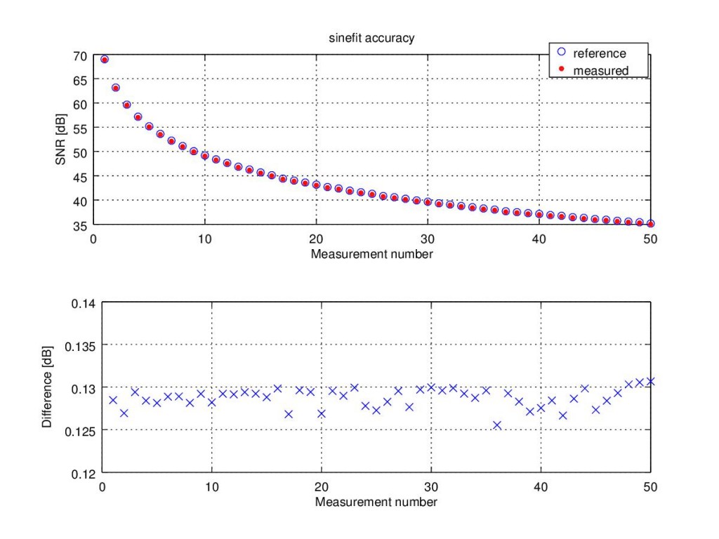
Maybe we should also check how well the sinefit method can estimate the SNR. Let’s create a small test bench for evaluating the estimation accuracy. The idea here is to create a known sine signal and a known noise signal so that we know the exact SNR and then sum up the two signals and use the sinefit function to estimate the SNR.

function tb_sinefit

close all

sampleRate=125e6;
Ts=1/sampleRate;
nSamples=16384;
t=(0:nSamples-1)*Ts;
f=20e3;

% reference signal
signal=real(exp(1j*2*pi*f*t));
rmsSignal=rms(signal);

nMeasurements = 50;
for iMeasurement=1:nMeasurements

    noiseLevel=0.00025*iMeasurement;

    % reference noise
    noise=noiseLevel*randn(1,nSamples);
    rmsNoise=rms(noise);
    % reference SNR
    refSNR(iMeasurement) = 20*log10(rmsSignal/rmsNoise);

    % estimate SNR from the noisy signal
    noisySignal = signal + noise;
    measuredSNR(iMeasurement) = ...
        calculateSNR(noisySignal, f, sampleRate);
end

compareSNR(refSNR,measuredSNR);

end

function compareSNR(refSNR,measuredSNR)

    subplot(2,1,1)
    plot(refSNR,'bo')
    hold on
    plot(measuredSNR,'r.')
    legend('reference','measured')
    grid
    ylabel('SNR [dB]')
    xlabel('Measurement number')
    title('sinefit accuracy')

    subplot(2,1,2)
    difference = refSNR-measuredSNR;
    plot(difference,'bx');
    grid
    ylabel('Difference [dB]')
    xlabel('Measurement number')
    minDiff = floor(min(difference)*100)/100;
    maxDiff = ceil(max(difference)*100)/100;
    a = axis;
    axis([a(1:2) minDiff maxDiff])

end

function y = rms(x)
y = norm(x)/sqrt(length(x));
end

The results are shown below. The estimated SNR is very close to the reference value. The difference is about 0.13dB (looks like the estimated SNR is consistently slightly smaller than the actual value).